When Is Your Test Result Significant The Statistics Behind The Ab Test

Management Summary
“Don’t trust any statistics you haven’t falsified yourself,” Winston Churchill most likely never said. However, you often hear this sentence in everyday life when the validity of statistical results is questioned. And in fact: it never hurts to know how such a result came about, especially if you do it yourselfA/B testingfor conversion optimization.
In the endless expanses of the Internet there are numerous online calculators that determine whether the difference between the conversion rates of two test variants is significant. Also withour significance calculatorsee at a glance which result is significant and which uplift or downlift could have occurred by chance.
However, we want to take a look at how these computers work. In this sense: “Don’t trust any statistics that you haven’t calculated yourself!”
Step 1: Observed and expected values
Most significance calculators use chi for their calculation2-Test (pronounced: ki-square). How this works and how it is calculated will be shown here using a fictitious example:
| Visitors | Conversions | Conversion rate | |
|---|---|---|---|
| Variant A | 9,998 | 1,001 | 10.01% |
| Variant B | 10,001 | 1,087 | 10.87% |
The conversion rates are obtained by dividing the observed conversions of a variant by the total number of visitors to a variant and multiplying them by 100%. For variant A this results in a conversion rate of 10.01% and for variant B 10.87%. The measure by which variant B performs better than variant A is called the uplift. This is calculated as follows: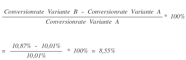 So variant B has an 8.55% higher conversion rate than variant A.However, this does not automatically mean that variant B is better than variant A.The different conversion rates can also arise by chance. This random deviation is called “statistical noise”.
For example, if you throw a die 600 times, you can expect the six to fall 100 times. In fact, there is a very high probability that we will observe a value that deviates from this. Maybe six is rolled 110 times, maybe just 92 times. Only if we roll an infinite number of dice can we be sure that exactly one sixth of all rolls will show a 6.
However, since an infinite number of observations is practically impossible, we must accept that the observed value may differ from the actual value. In order to be able to judge whether variant B actually performs better than variant A, we have to find out how likely the difference is due to statistical noise.
To do this, a crosstab is created that contains the observed values of converted and non-converted visitors:
| Visitors | Conversions | No conversions | Conversion rate | |
|---|---|---|---|---|
| Variant A | 9,998 | 1,001 | 8,997 | 10.01% |
| Variant B | 10,002 | 1,087 | 8,915 | 10.87% |
The next step is to compare these observed values with the values that one would expect if there were no difference between the two variants. The expected values result from the common conversion rate of both variants: The number of visitors to each variant is now multiplied with this common conversion rate. This gives us the expected conversions of a variant:
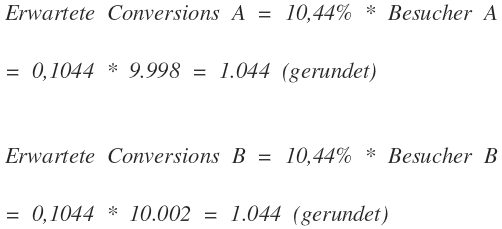 The expected non-conversions are easily determined by subtracting the expected conversions from the number of visitors of the two variants:
 We now enter these values into our crosstab:
| Visitors | Conversions | No conversions | CR | |||
|---|---|---|---|---|---|---|
| observed | expected | observed | expected | |||
| Variant A | 9,998 | 1,001 | 1,044 | 8,997 | 8,954 | 10.01% |
| Variant B | 10,002 | 1,087 | 1,044 | 8,915 | 8,958 | 10.87% |
Step 2: Calculate deviation values
Now we calculate the deviation from the expected value for each observed value. This is done with the formula: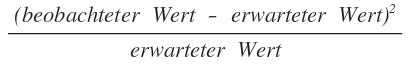 By squaring the deviation, we ensure that it does not matter whether the observed value is below or above the expected value and avoid positive and negative deviations canceling out or weakening each other. In addition, larger deviations are taken into account more than small deviations.
By dividing by the expected value, we also accept a slightly larger deviation for higher expected values than for lower expected values.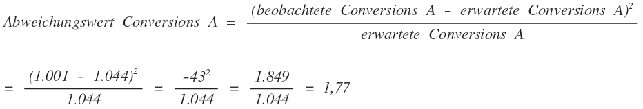 We proceed similarly for the conversions of variant B and the values of the non-conversions. We now add all four values together and get the test value for the Chi2-Test:
![]()
Step 3: Check for significance
In general, the higher this value is, the higher the probability that the two variants actually differ. It is not possible to make a 100% statement about this, so a confidence value must be chosen. This indicates the probability that the two variants are different. For this confidence value you now hit in oneChi2-Distribution tablehow high the test value must be at least so that a difference between the two variants is at least as high as the confidence value. Popular confidence values and the associated minimum test values are:
| Confidence | Minimum test value | note |
|---|---|---|
| 90% | 2.71 | tends to |
| 95% | 3.84 | significant |
| 99% | 6.63 | very significant |
| 99.9% | 10.83 | highly significant |
We decide on a confidence of 95%, for this we need a test value of at least 3.84. With 3.955 we skip this minimum value, so we can claim with 95% probability:Variants A and B differ significantly from each other. The measured uplift actually has its origin in a higher conversion rate and is not just caused by statistical noise.However, what we cannot say for sure is that the uplift is actually +8.55%. This is the most likely value that the uplift can take, but it is also subject to statistical noise. But it is very likely close to this value.
Is all this too complicated for you? Then just use thate-dialog significance calculator >